Introduction

A particularly brutal aspect of real-time rendering in AR environments is that your object is directly exposed to the physical reality around it for comparison. Unlike your typical game-engine, masking or hiding physical inaccuracies in the model used to simulate real reflection of light on your virtual object is not going to work very well when all the other objects on screen somehow behave differently. If the augmented object doesn’t match up with reality, a knee-jerk reaction is to edit the responsible shader and simply tweak the output with a bunch of random multipliers until all looks right again. However, before all the magic-number adjustments get out of hand, it might be time to review the basics and avoid a non-physically-based-shading-post-traumatic-stress-disorder™.

Many real-time engine writers have concentrated on getting their equations right. The most recent result is the Siggraph Physically Based Shading Course (2012 Edition, 2013 Edition). I will roughly lay out the basic principles of PBS and refer to other very good online blogs which have covered most of the details that do not need to be repeated ad absurdum.

Consider the standard form of the rendering equation:

When shading your object, it is important that light reflection off the surface behaves physically plausible, that is the BRDF has to respect certain conditions:

• Positivity: the value of the BRDF is always positive.

• Energy conservation: the total amount of energy reflected over all directions of the surface must be less or equal to the total amount of energy incident to it. In practical terms this means that the visible energy (i.e. reflected light) can at best decrease after bouncing off a surface, while the rest turns to heat or some other form which isn’t part of the simulation. A non-emissive surface however cannot emit more light than it received.

• Helmholtz reciprocity: the standard assumption in geometric optics is that exchanging in- and outgoing light direction in the BRDF doesn’t change the outcome.

• Superposition: the BRDF is a linear function. Contribution of different light sources may be added up independently. There is a debate about whether this is a property of the BRDF or light.

It is usually the energy conservation in the specular term where things go wrong first. Without normalization Blinn-Phong for instance, a popular and easy way to model specular reflection, can easily be too bright with small specular powers and quickly loose too much energy when increasing the term.

But there is more! Many renderers assume that there are materials which are perfectly diffuse, i.e. they scatter incident light in all directions equally. There is no such thing. John Hable demonstrated this by showing materials which would be considered to be diffuse reflectors. You can read more in his article Everything has Fresnel.

So here we are, with a BRDF that can output too much energy, darkens too quickly and can’t simulate the shininess of real world objects because the model is built with unrealistic parameters. How do we proceed?

One solution is to find a normalization factor for Blinn-Phong to fix the energy issues with the model and add a Fresnel term. There are also several other reflection models to choose from: Oren-Nayar, Cook-Torrance, Ashikhmin-Shirley, Ward…

Microfacet Models

Physically based BRDF models are built on the theory of microfacets, which states that the surface of an object is composed of many tiny flat mirrors, each with its own orientation. The idea of a microfacet model is to capture the appearance of a macro-surface not by integration over its micro-factets, but by statistical means.

A microfacet model looks like this (with the notation for direct visibility):

where

This specular part of the BRDF has three important components:

• the Fresnel factor
• a geometric term
• a Normal Distribution Function (NDF)

The Fresnel term simulates the Fresnel behavior and can be implemented with the Schlick approximation.

The geometric term models the self-occlusion behavior of the microfacets on the surface and can be thought of as a visibility factor for a micro-landscape which simply depends on one parameter for the surface roughness.

The NDF is the term that gives you the distribution of microfacet normals across the surface from a certain point of view. If more microfacets are oriented in the half-vector direction , the specular highlight will be brighter. is the density of normals oriented in direction .

Conclusion

To sum up, the idea here is to start out with the correct shading model to avoid inconsistencies that might turn up later (I’m speaking out of negative experience tweaking arbitrary parameters of my old AR renderer). Turning to such a model might not produce visible differences immediately, but will later be noticeable once GI is added to the system where the light bounces multiply any error one made right at the start.

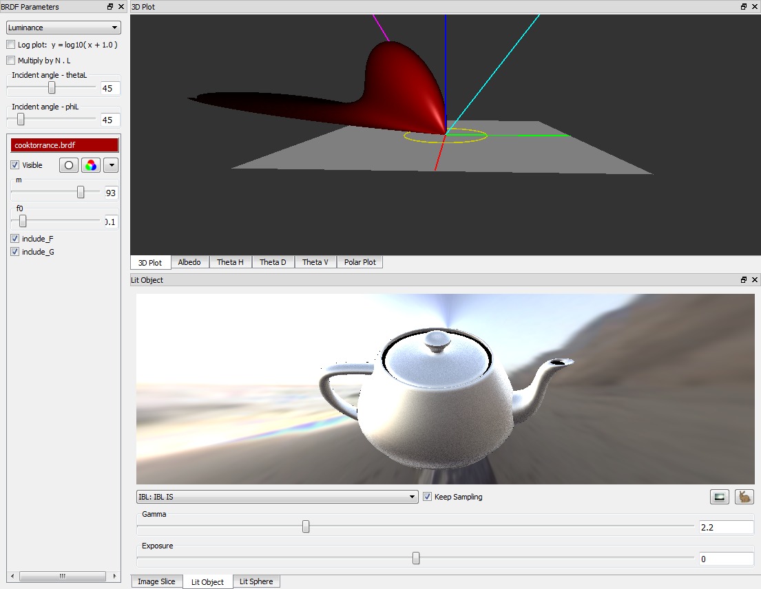
A neat way to check how you are on the reality-scale is Disney’s BRDF Explorer, which comes with GLSL implementations of several microfacet terms and other BRDFs (have a look at the brdf/ subdirectory and open one of the .brdf files).

You can download measured materials from the MERL database, load them in the BRDF Explorer and compare them to see how well analytical BRDFs match up to reality.

More References

1. Hill et al., Siggraph PBS 2012
2. Hill et al., Siggraph PBS 2013
3. Brian Karis, Specular BRDF Reference
4. John Hable, Everything has Fresnel
5. Rory Driscoll, Energy Conservation In Games
6. Rory Driscoll, Physically-Based Shading
7. Simon Yeung, Microfacet BRDF
8. Sébastien Lagarde, PI or not to PI in game lighting equation
9. Wikipedia, Schlick’s approximation
10. Christian Schüler, The Blinn-​Phong Normalization Zoo
11. D3D Book, Cook-Torrance
12. Disney, BRDF Explorer
13. MERL, MERL BRDF Database